本文共 5245 字，大约阅读时间需要 17 分钟。

蒙特卡洛模拟

蒙特卡洛模拟是金融学和数值科学中最重要的算法之一。它之所以重要，是因为在期权定价或者风险管理问题上有很强的能力。和其它数值方法相比，蒙特卡洛方法很容易处理高维问题，在这种问题上复杂度和计算需求通常以线性方式增大。

蒙特卡洛方法的缺点是：它本身是高计算需求的，即使对于相当简单的问题也往往需要海量的计算。因此，必须高效的实现蒙特卡洛算法。

下面使用不同的方法实现蒙特卡洛算法

1.Scipy

2.纯Python

3.向量化Numpy

4.全向量化Numpy

方法一：Scipy

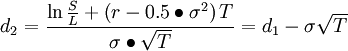
欧式看涨期权的定价公式Black-Scholes-Merton(1973):

其中：

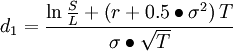
C—期权初始合理价格

L—期权交割价格

S—所交易金融资产现价

T—期权有效期

r—连续复利计无风险利率

σ2—年度化方差

N()—正态分布变量的累积概率分布函数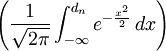

# 导用到的库from math import log, sqrt, expfrom scipy import stats

# 期权的定价计算,根据公式１．def bsm_call_value(S_0, K, T, r, sigma):    S_0 = float(S_0)    d_1 = (log(S_0 / K) + (r + 0.5 *sigma **2) *T)/(sigma * sqrt(T))    d_2 = (log(S_0 / K) + (r - 0.5 *sigma **2) *T)/(sigma * sqrt(T))    C_0 = (S_0 * stats.norm.cdf(d_1, 0.0, 1.0) - K * exp(-r * T) * stats.norm.cdf(d_2, 0.0, 1.0))    return C_0

# 计算的一些初始值S_0 = 100.0    # 股票或指数初始的价格;K = 105        #  行权价格T = 1.0        #  期权的到期年限(距离到期日时间间隔)r = 0.05       #   无风险利率sigma = 0.2    # 波动率(收益标准差)

# 到期期权价值%time print (bsm_call_value(S_0, K, T, r, sigma))

8.021352235143176Wall time: 511 µs

方法二：Python

下面的计算仍基于BSM(balck-scholes-merton),模型中的高风险标识(股票指数)在风险中立的情况下遵循以随机微分方程(SDE)表示的布朗运动．

# 导入python模块from time import timefrom math import exp, sqrt, logfrom random import gauss, seed

seed(2000)# 计算的一些初始值S_0 = 100.0    # 股票或指数初始的价格;K = 105        #  行权价格T = 1.0        #  期权的到期年限(距离到期日时间间隔)r = 0.05       #   无风险利率sigma = 0.2    # 波动率(收益标准差)M = 50         # number of time stepsdt = T/M       # time entervalI = 20000       # number of simulation

start = time()S = []     # for i in range(I):    path = []    # 时间间隔上的模拟路径    for t in range(M+1):        if t==0:            path.append(S_0)        else:            z = gauss(0.0, 1.0)            S_t = path[t-1] * exp((r-0.5*sigma**2) * dt + sigma * sqrt(dt) * z)            path.append(S_t)    S.append(path)# 计算期权现值C_0 = exp(-r * T) *sum([max(path[-1] -K, 0) for path in S])/Itotal_time = time() - startprint ('European Option value %.6f'% C_0)print ('total time is %.6f seconds'% total_time)

European Option value 8.159995total time is 1.616999 seconds

前三十条模拟路径

# 选取部分模拟路径可视化import matplotlib.pyplot as plt %matplotlib inline plt.figure(figsize=(10,7))plt.grid(True)plt.xlabel('Time step')plt.ylabel('index level')for i in range(30):    plt.plot(S[i])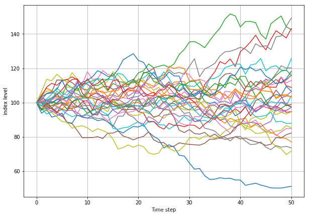

方法三： 向量化的Numpy

使用numpy的一些数组，来减少运算

# 导入模块import numpy as npfrom time import time

# 计算的一些初始值S_0 = 100.0    # 股票或指数初始的价格;K = 105        #  行权价格T = 1.0        #  期权的到期年限(距离到期日时间间隔)r = 0.05       #   无风险利率sigma = 0.2    # 波动率(收益标准差)M = 50         # number of time stepsdt = T/M       # time entervalI = 20000       # number of simulation

# 20000条模拟路径，每条路径５０个时间步数S = np.zeros((M+1, I))S[0] = S_0np.random.seed(2000)start = time()for t in range(1, M+1):    z = np.random.standard_normal(I)    S[t] = S[t-1] * np.exp((r- 0.5 * sigma **2)* dt + sigma * np.sqrt(dt)*z)C_0 = np.exp(-r * T)* np.sum(np.maximum(S[-1] - K, 0))/Iend = time()

# 估值结果print ('total time is %.6f seconds'%(end-start))print ('European Option Value %.6f'%C_0)

total time is 0.039680 secondsEuropean Option Value 7.993282

前２０条模拟路径

# 前２０条模拟路径import matplotlib.pyplot as plt%matplotlib inline plt.figure(figsize=(10,7))plt.grid(True)plt.xlabel('Time step')plt.ylabel('index level')for i in range(20):    plt.plot(S.T[i])

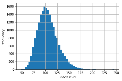
到期指数模拟水平

# 到期时所有模拟指数水平的频率直方图%matplotlib inlineplt.hist(S[-1], bins=50)plt.grid(True)plt.xlabel('index level')plt.ylabel('frequency')

Text(0, 0.5, 'frequency')

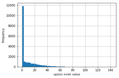
到期期权内在价值

# 模拟期权到期日的内在价值%matplotlib inlineplt.hist(np.maximum(S[-1]-K, 0), bins=50)plt.grid(True)plt.xlabel('option inner value')plt.ylabel('frequency')

Text(0, 0.5, 'frequency')

方法四：全向量化的Numpy

import numpy as npfrom time import time

# 计算的一些初始值S_0 = 100.0    # 股票或指数初始的价格;K = 105        #  行权价格T = 1.0        #  期权的到期年限(距离到期日时间间隔)r = 0.05       #   无风险利率sigma = 0.2    # 波动率(收益标准差)M = 50         # number of time stepsdt = T/M       # time entervalI = 20000       # number of simulation

np.random.seed(2000)start = time()# 生成一个随机变量的数组，M+1行，I列# 同时计算出没一条路径，每一个时间点的指数水平的增量# np.cumsum(axis=0)，在列的方向上进行累加得到每一个时间步数上的指数水平S = S_0 * np.exp(np.cumsum((r - 0.5*sigma **2) *dt +sigma *np.sqrt(dt) *np.random.standard_normal((M+1, I)),axis=0))S [0] = S_0C_0 = np.exp(-r * T) * np.sum(np.maximum(S[-1] - K, 0))/Iend = time()

print ('toatl time is %.6f seconds'%(end-start))print ('Europaen Option Value %.6f'%C_0)

toatl time is 0.077348 secondsEuropaen Option Value 8.113643

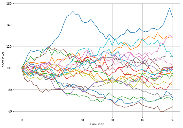
前２０条模拟路径

# 前２０条模拟路径import matplotlib.pyplot as plt%matplotlib inline plt.figure(figsize=(10,7))plt.grid(True)plt.xlabel('Time step')plt.ylabel('index level')plt.plot(S[:,:20])

[
   
    , 
    
     , 
     
      , 
      
       , 
       
        , 
        
         , 
         
          , 
          
           , 
           
            , 
            
             , 
             
              , 
              
               , 
               
                , 
                
                 , 
                 
                  , 
                  
                   , 
                   
                    , 
                    
                     , 
                     
                      , 
                      
                       ]
                      
                     
                    
                   
                  
                 
                
               
              
             
            
           
          
         
        
       
      
     
    
   

模拟到期指数水平

# 到期时所有模拟指数水平的频率直方图import matplotlib.pyplot as plt%matplotlib inlineplt.hist(S[-1], bins=50)plt.grid(True)plt.xlabel('index level')plt.ylabel('frequency')

Text(0, 0.5, 'frequency')

模拟到期期权内在价值

# 模拟期权到期日的内在价值%matplotlib inlineplt.hist(np.maximum(S[-1]-K, 0), bins=50)plt.grid(True)plt.xlabel('option inner value')plt.ylabel('frequency')

Text(0, 0.5, 'frequency')

sum(S[-1] < K)    # 在两万次模拟中超过一万次到期期权内在价值为０

10748

结果对比

1.Scipy,估值结果：8.021352，耗时：511 µs

2.Python,估值结果：8.159995，耗时：1.616999s

3.向量化Numpy,估值结果：7.993282，耗时：0.039680s

4.完全向量化Numpy,估值结果：8.113643，耗时：0.077348

Scipy，用时最短是因为，沒有进行20000次的模拟估值．其他三个方法进行了20000次的模拟，基于Numpy的计算方法速度比较快．

转载地址：http://sdzdf.baihongyu.com/